In this article (and video above), we tackle a key concept from the Engineering Economics section of the FE Exam: PW Problems analysis. We’re given an investment with an initial cost and varying cash inflows over six years, and we calculate its value using an 8% interest rate. To do this, we apply the Single Payment Present Worth formula, which is ideal for handling non-uniform cash flows. Mastering this method is essential, as it’s a common topic you can expect to encounter on the FE Exam.
Question:
An investment generates the following cash flows over a 6-year period. Determine the Present Worth (PW) of the investment using an annual interest rate of 8%.
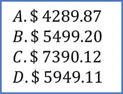
In today’s question, we are presented with a series of cash flows occurring over the span of 6 years. The investment has an initial cost of $30,000 in year zero, followed by a series of positive cash flows. Here, the goal is to calculate the Present Worth (PW) of these cash flows at an 8% interest rate. However, since these cash flows occur at different points in time, we’ll also need to account for the time value of money. Let’s start with a basic review of the concepts behind this problem:
The Present Worth Method:
The Present Worth method is a tool in engineering economics used to evaluate the total value of a series of future cash flows as if they occurred at the present time.
Time Value of Money:
The concept that a sum of money is worth more today than at a future date due to its earning potential
Engineering Economics Formulas:
The FE Handbook provides us with a set of different formulas we can apply depending on the type of cash flow pattern we are presented with. If the cash flows are the same each year, we can use the Uniform Series Present Worth formula. On the other hand, if the cash flows increase by a fixed amount each year, we use the Uniform Gradient Present Worth formula. When the cash flows are different each year with no repeating pattern, we’ll use the Single Payment Present Worth formula to discount each cash flow individually before adding them together to find the total Present Worth of the investment.
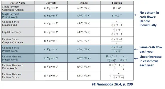
The Single Payment Present Worth Formula:
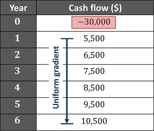
Take a look at the cash flows we are presented with. Although the cash flows increase uniformly
from the first year onward, the presence of an initial $30,000 cost at year zero would require us to account for it separately. While the Uniform Gradient formula could apply to the increasing portion of the cash flows, using the Single Payment formula on each cash flow individually would result in the simplest and most straightforward method for this problem. This is because it typically works in all cases, requires no pattern recognition, and simply discounts each cash flow individually with the same straightforward calculation.
The Single Payment Present Worth formula is given by:
\( \displaystyle \frac{P}{F} = (1 + i)^{-n} \)
Where represents the present value, is the future value, is the interest rate per period, and is the number of periods. The formula allows us to calculate the present value of a single future cash flow.
When we have multiple cash flows occurring at different times, we simply apply this formula to each cash flow individually and sum the results to find the total present worth:
\( \displaystyle P = \sum_{n=0}^{N} \frac{F}{(1 + i)^{-n}}. \)
We can directly apply this equation to solve for our investment’s present worth. We start with the initial cost of $30,000 in year zero, which doesn’t need to be discounted since it’s already at the present time. Then, for each of the future cash flows from years 1 through 6, we apply the formula:
\( \displaystyle
\rightarrow P = \frac{F_0}{(1 + i)^0} + \frac{F_1}{(1 + i)^1} + \ldots + \frac{F_6}{(1 + i)^6}
\)
\( \displaystyle
\rightarrow P = \frac{-30\,000}{(1 + 0.08)^0}
+ \frac{5500}{(1 + 0.08)^1}
+ \frac{6500}{(1 + 0.08)^2}
+ \frac{7500}{(1 + 0.08)^3}
+ \frac{8500}{(1 + 0.08)^4}
+ \frac{9500}{(1 + 0.08)^5}
+ \frac{10500}{(1 + 0.08)^6}
\)
\( \displaystyle
\rightarrow P = -30000 + 5092.59 + 5572.70 + 5953.74 + 6247.75 + 6465.54 + 6616.78
\)
\( \displaystyle
\rightarrow \boldsymbol{P = \$5949.10}
\)
We calculate the present value of each cash flow by substituting these values into a calculator. Once we’ve discounted each cash flow to its present value, we add them all together. Based on this calculation, the Present Worth of the investment is approximately $5,949.10. This value tells us the total worth of the investment today after accounting for the time value of money for future payments at an 8% interest rate.
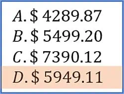
And that wraps up our problem! Comparing our calculated Present Worth to the answer choices, we see that our result is closest to Option D. While our step-by-step calculations may involve some rounding or truncated values along the way, using the full values directly in your calculator should give you a result of exactly $5,949.11.
To summarize, today we tackled PW Problems involving an initial investment of $30,000 followed by a series of increasing cash flows over 6 years. After reviewing key economic principles and formulas from the FE Handbook, we determined that the Single Payment Present Worth formula was the most reliable method to apply since it handles any cash flow pattern by discounting each value individually.
By applying this formula to each year’s cash flow and summing the results, we calculated the total present value of the investment to be approximately $5,949.10. This process highlights how we can apply the time value of money to evaluate future cash flows in today’s terms, an essential skill in engineering economics.
I hope you found this week’s FE Exam article helpful. In upcoming articles, I will answer more FE Exam questions and run through more practice problems. We publish videos bi-weekly on our Pass the FE Exam YouTube Channel. Be sure to visit our page here and click the subscribe button as you’ll get expert tips and tricks – to ensure your best success – that you can’t get anywhere else. Believe me, you won’t want to miss a single video.
Lastly, I encourage you to ask questions in the comments of the videos or here on this page, and I’ll read and respond to them in future videos. So, if there’s a specific topic you want me to cover or answer, we have you covered.
I’ll see you next week… on Pass the FE Exam
Anthony Fasano, P.E., AEC PM, F. ASCE

Leave a Reply